CodinGame: Best fit to data - Rust - Regression Analysis
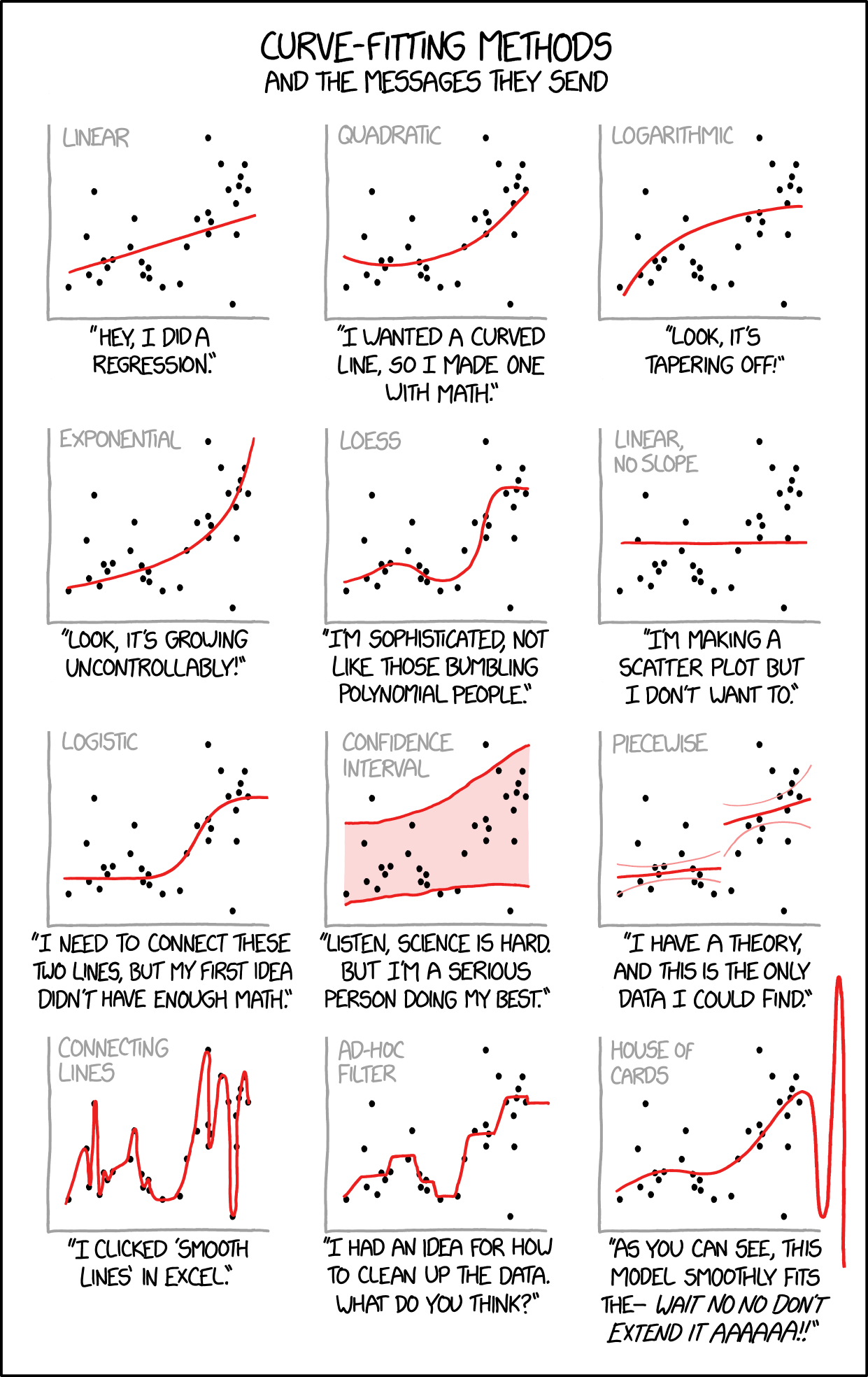
Linear and logarithmic regressions were derived here. Models were fitted in rust language. This article shows that sometimes it's worth improving the theoretical model before starting implementation.


We will discuss exercise:

Goal is find best fitting model for given dataset. For example for data:
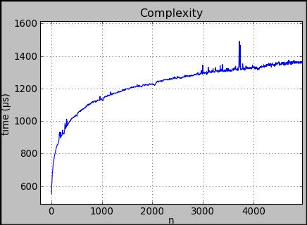
we should print O(log n). We can select models from list:
- O(1),
- O(log n),
- O(n),
- O(n log n),
- O(n^2),
- O(n^2 log n),
- O(n^3),
- O(2^n)
Input of program will contain first line with number of next lines and any following line will contain n and t values.
There are constrains:
5 < N < 1000
5 < num < 15000
0 < t < 10000000
and exemplary input:
10
5 341
1005 26324
2005 52585
3005 78877
4005 104925
4805 125920
6105 159156
7205 188017
8105 211417
9905 258991
should give to us
O(n)because of is is similar to linear growth.
Least Square Fitting
We can derive equation on coefficient and assuming that we want to minimize sum of second powers of differences between measurement and prediction of our model.
$$ R^2 = \sum_i \left( t_i - f(n_i, a) \right)^2 $$This approach is called least squares fitting, and you can read more about it on MathWorld

Minimal value means that partial derivative by parameter of model a is 0.
Linear Regression
Now we can assume that function is linearly dependent from scaling parameter a.
Our goal is find equation to compute a and then R^2. Our derivative can be simplified:
Using last equation from Linear Square Fitting we can compute a
so
$$ a = \frac{\sum_i t_i f(n_i)}{\sum (f(n_i))^2 } $$and
$$ R^2 = \sum_i \left( t_i - a f(n_i) \right)^2 $$Our equations looks beautifully but the devil is in the details.
If we will look at constrains of data for this exercise:
5 < N < 1000
5 < num < 15000
0 < t < 10000000
and remember models that we need to test it is easy too see that we will operate on huge numbers.
For example 2^n with n = 15 000 is much more than max range of 64 bit float

that is constrained to 2^1024. There are tricks that allow to operate on these ranges, but instead of hacking computers constrains we will use math.
Instead of operating on big numbers we will use their logarithm to computation.
Logarithmic Regression
Our solution is consequence of observation that if we will match logarithms of models to logarithms of t data then in result will will select the same model.
So adding log both to data and function we getting equation:
rewriting this equation we can obtain a
where
$$ N = \sum_i 1 $$and rewriting equation for R^2 we see:
Lets introduce new variable c defined as
and then R^2 can be rewritten as
we can see that now there is no chance to operate on too big numbers so we can start implementation of these equations.

Reading series of data from standard input
Lets start from definition of Point structure that represents single measurement.
#[derive(Debug)]
struct Point {
    n: u32,
    t: u32,
}
in main we will read standard input to String named buffer.
fn main() {
    let mut buffer = String::new();
    std::io::stdin().read_to_string(&mut buffer).unwrap();
}
we want to process this buffer and obtain vector of Points. To do it we writing function:
fn read_series(input: String) -> Vec<Point> {
    let mut iterator = input.lines();
    let n = iterator.next();
    let mut res: Vec<Point> = vec![];

    if Some(n).is_some() {
        for line in iterator {
            if let Some((n, y)) = line.split_once(' ') {
                res.push(Point {
                    n: n.parse::<u32>().unwrap_or(0),
                    t: y.parse::<u32>().unwrap_or(0),
                });
            }
        }
        return res;
    }

    return vec![];
}
we can check if it works adding to main line
println!("{:?}", read_series(buffer));Computing sum on series using closure
In presented equations we had some sums, so to simplify further code lets implement sum function that can use closures to define operation what should be summed.
I initially wrote it as noob
fn sum(series: &Vec<Point>, expression: impl Fn(&Point) -> f64) -> f64 {
    let mut res = 0f64;
    for point in series {
        res += expression(point)
    }
    res
}
but soon fixed as hacker
fn sum(series: &Vec<Point>, expression: impl Fn(&Point) -> f64) -> f64 {
    series.into_iter().fold(0f64, |acc, point| { acc + expression(point) })
}
we can add test
#[cfg(test)]
mod tests {
    use crate::{Point, sum};

    #[test]
    fn sum_test() {
        assert_eq!(sum(
            &vec![Point { n: 0u32, t: 1u32 }, Point { n: 1u32, t: 2u32 }],
            |p: &Point| { f64::from(p.t) },
        ), 3f64);
    }
}
Evaluating Sum of Least Squares
Our models to test can be represented using structure
struct Model {
    name: String,
    fn_log: fn(u32) -> f64,
}
but after computing R^2 we can save result as
struct EvaluatedMode {
    name: String,
    r2_log: f64,
}
this is convenient data organization because results of evaluation will be compared by r2_log but then name should be available to print as output.
Due to this reason we will select following signature for R^2 evaluation
fn evaluate_r2(model: Model, series: &Vec<Point>) -> EvaluatedModeSeries is passed by reference similarly like in sum. We do not want to change them or copy so operating on reference is preferred option for us.
Rewriting equations derived before to rust we can implement in this way
fn evaluate_r2(model: Model, series: &Vec<Point>) -> EvaluatedMode {
    let Model { name, fn_log } = model;
    let c = 1.0 / series.len() as f64 * sum(
        &series,
        |p| { f64::ln(f64::from(p.t)) - fn_log(p.n) },
    );
    let r2_log = sum(
        &series,
        |p| f64::powi(f64::ln(f64::from(p.t)) - fn_log(p.n) - c, 2),
    );
    EvaluatedMode {
        name,
        r2_log,
    }
}
Selection best fitting model
To select model we starting from function signature
fn select_model(series: &Vec<Point>) -> String {and defining vector with models possible to select. Instead of original functions we adding fn_log what are logharithms of these functions.
    let models: Vec<Model> = vec![
        Model {
            name: String::from("O(1)"),
            fn_log: |_n| 0f64,
        },
        Model {
            name: String::from("O(log n)"),
            fn_log: |n| f64::ln(f64::ln(f64::from(n))),
        },
        Model {
            name: String::from("O(n)"),
            fn_log: |n| f64::ln(f64::from(n)),
        },
        Model {
            name: String::from("O(n log n)"),
            fn_log: |n| f64::ln(f64::from(n)) + f64::ln(f64::ln(f64::from(n))),
        },
        Model {
            name: String::from("O(n^2)"),
            fn_log: |n| 2.0 * f64::ln(f64::from(n)),
        },
        Model {
            name: String::from("O(n^2 log n)"),
            fn_log: |n| 2.0 * f64::ln(f64::from(n)) + f64::ln(f64::ln(f64::from(n))),
        },
        Model {
            name: String::from("O(n^3)"),
            fn_log: |n| 3.0 * f64::ln(f64::from(n)),
        },
        Model {
            name: String::from("O(2^n)"),
            fn_log: |n| f64::from(n) * f64::ln(2.0),
        },
    ];
finally we mapping these models to evaluated models and reducing result to model with smallest r2_log
    models.into_iter().map(|m| { evaluate_r2(m, series) }).reduce(|p, n| {
        if p.r2_log < n.r2_log { p } else { n }
    }).unwrap().name
}
its everything. Now we can change last line of main to
println!("{}", select_model(&read_series(buffer)));
and our program works.
Traditionally you can check full code with test on my github
 gustawdaniel